Recognizing rules, patterns and correlations from transaction data
If we have typical retail transaction data, we can apply different data science methods and algorithms to discover rules, patterns and correlations that exist within the data. For example:
- If a customer bought product1 and product2, very often he also bought product3.
- Product1 and product2 are “similar”: they cost approximately the same, they are sold in approximately the same quantities, they are sold in similar points of sale.
- Points of sale are “similar”: their income is approximately the same, they sell mostly products from the same category, they buy mostly from the same wholesaler.
- Sales of some products or categories of products are tied to a season of the year.
Using these rules and patterns, one can make quality business decisions and thus increase sales, income, customer retention or reduce the unnecessary expenses.
Data science could be explained as audit and research of big amounts of data with the goal of finding rules like above and answering business related questions. It includes many different science, engineering and business areas:
- Mathematics and statistics.
- Programming and information technologies.
- Econometry, marketing, business intelligence.
Thus to manage data science one has to cover a wide area of theory, practical skills and targeted reasoning.
Wholesaler/Retailer Transactions Example
The best way to introduce the complexity and the power of data science is to start with an example.
We will use a simulated transaction data between a set of wholesalers and retailers in a period of 5 years. The data consists of transactions that include:
- transaction identifier (invoice number or similar)
- wholesaler identifier (name, assuming that it is unique)
- wholesaler location (town, city, province)
- product identifier (name, assuming that it is unique)
- product category (based on product type, usage)
- manufacturer identifier (name, assuming that it is unique)
- retailer identifier (name, assuming that it is unique)
- retailer location (town, city, province)
- date (date of sales)
- unit price (product unit price for the transaction)
- quantity (amount of product purchased in the transaction)
- price (total price for the transaction)
##   TransactionID    WholesalerID WholesalerLocation    ProductID
## 1      21106905 veleprodaja_008             Osijek proizvod_121
## 2      21106905 veleprodaja_001             Zagreb proizvod_033
## 3      21106905 veleprodaja_005             Zagreb proizvod_101
## 4      21106905 veleprodaja_006              Zadar proizvod_198
## 5      21106905 veleprodaja_009             Osijek proizvod_143
##   ProductCategory  ManufacturerID      RetailerID RetailerLocation
## 1  kategorija_001 proizvodjac_018 maloprodaja_001         Krizevci
## 2  kategorija_005 proizvodjac_015 maloprodaja_001         Krizevci
## 3  kategorija_005 proizvodjac_004 maloprodaja_001         Krizevci
## 4  kategorija_005 proizvodjac_003 maloprodaja_001         Krizevci
## 5  kategorija_005 proizvodjac_027 maloprodaja_001         Krizevci
##         Date UnitPrice Quantity   Price
## 1 2014-01-01     17.34   208.00 3606.72
## 2 2014-01-01      8.36    35.00  292.60
## 3 2014-01-01     12.87    39.00  501.93
## 4 2014-01-01      8.45    39.00  329.55
## 5 2014-01-01 9.41 33.00 310.53Note: each data entry (“row”) is bound to one product. So, if a typical purchase/transaction includes more different products, then more entries in our sample table (one per each different product bought in a transaction) will have the same transaction identifier. This is one way of encoding transactions to simplify the data management, but it is not restricting in any way because every set of transaction data can be encoded like this.
## transactions in sparse format with
##  11997 transactions (rows) and
##  200 items (columns)
We have a total of 11997 transactions with 200 products.
Buying rules/patterns
Let’s see if we can derive some rules (patterns) on products often bought together. We will look for the rules for the products that occur in at least 0.1% of transactions and that occur together in at least 70% of common transactions.
## set of 116 rules
##
## rule length distribution (lhs + rhs):sizes
##   4
## 116
##
##    Min. 1st Qu.  Median    Mean 3rd Qu.    Max.
##       4       4       4       4       4       4
##
## summary of quality measures:
##     support           confidence          lift           count
##  Min.   :0.003918   Min.   :0.7000   Min.   :2.645   Min.   :47.00
##  1st Qu.:0.005335   1st Qu.:0.7023   1st Qu.:2.762   1st Qu.:64.00
##  Median :0.005960   Median :0.7083   Median :2.806   Median :71.50
##  Mean   :0.005970   Mean   :0.7100   Mean   :2.812   Mean   :71.62
##  3rd Qu.:0.006585   3rd Qu.:0.7143   3rd Qu.:2.849   3rd Qu.:79.00
##  Max.   :0.008169   Max.   :0.7436   Max.   :3.009   Max.   :98.00
##
## mining info:
##                    data ntransactions support confidence
##  retailtransactions_use         11997   0.001        0.7
We have found 116 rules with the given parameters. Rules consist of the left hand side (lhs – “condition”) and right hand side (rhs – “consequence”). Let’s see some of the rules:
##     lhs               rhs                support confidence     lift count
## [1] {proizvod_014,
##      proizvod_161,
##      proizvod_162} => {proizvod_073} 0.008168709  0.7101449 2.848415    98
## [2] {proizvod_033,
##      proizvod_058,
##      proizvod_145} => {proizvod_077} 0.008002001  0.7218045 2.819762    96
## [3] {proizvod_079,
##      proizvod_084,
##      proizvod_142} => {proizvod_116} 0.007668584  0.7131783 2.864412    92
## [4] {proizvod_090,
##      proizvod_137,
##      proizvod_138} => {proizvod_054} 0.007501875  0.7086614 2.733701    90
## [5] {proizvod_043,
##      proizvod_187,
##      proizvod_200} => {proizvod_171} 0.007418521  0.7295082 2.821376    89
Left hand sides of the rules contain “conditional” products and right hand sides contain “consequential” products. For example (rule 1): if someone buys proizvod_014, proizvod_161 and proizvod_162 then he will buy proizvod_073 with a probability of 71% (confidence).
Possible benefits from this information:
- offer together products related by the rules and increase sales
- promote together products related by the rules and increase promotion effect
- offer a discount if products related by the rules are bought together and increase sales
Time related patterns
When we have time structured sales data (for example transaction data with dates and times like in our example), we can investigate general and seasonal trends in the sales. Below is a time series graph of total sales related to one product category.
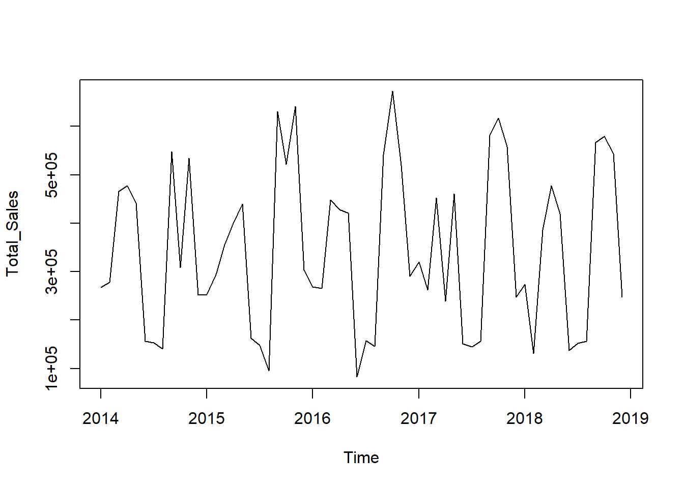
When we separate the general trend and seasonal effect, we get the following graphs:
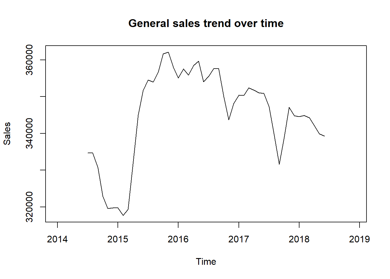
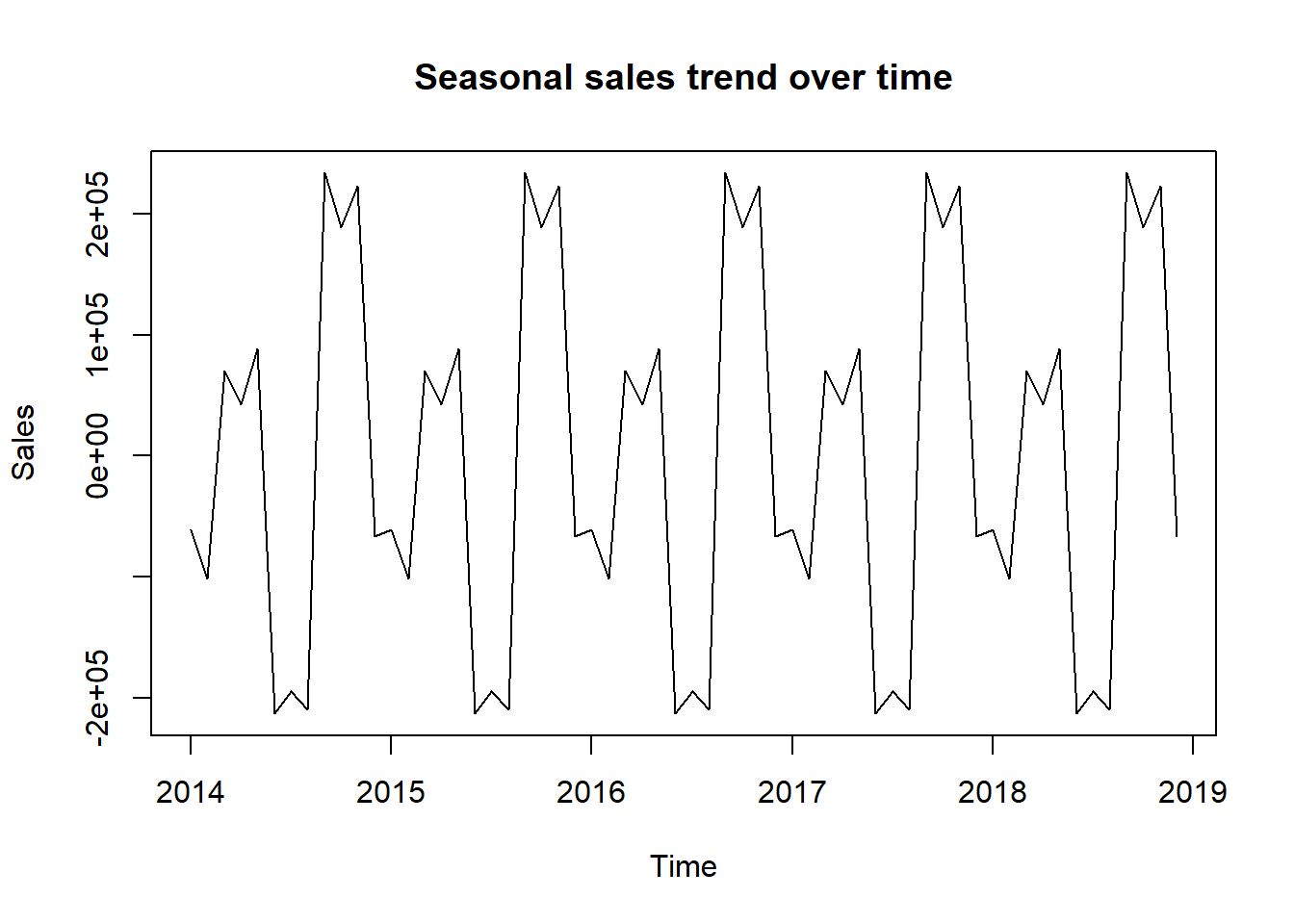
It is easily seen from the graph above that the sales goes up close to the beginning and close to the end of the year, and drops in the middle of the year.
Possible benefits from this information:
- offer and promote the most sought products in a certain season and increase sales
- reduce offering of the least sought products in a certain season and decrease expenses
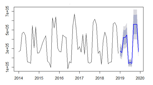
Using the past sales information and its trends, we can make a prediction on the future sales.
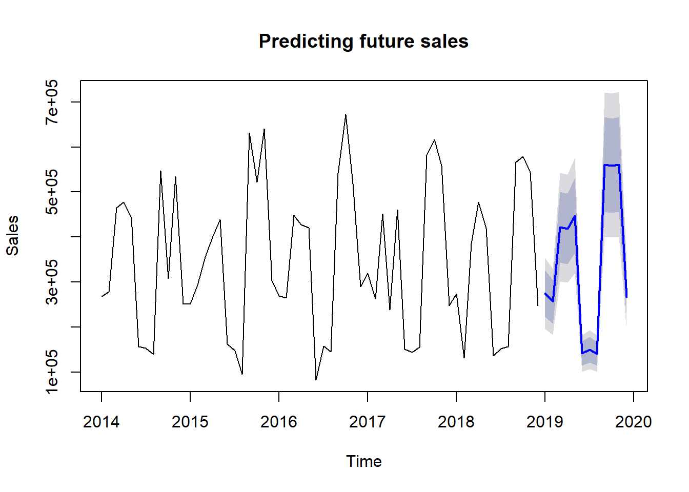
Possible benefits from this information:
- plan marketing and sales activities in advance, decrease expenses and increase sales
- increase or decrease production to cover the predicted market needs
Finding similarities and grouping data
When investigating products, it is interesting to find which are similar in the sense of income and number of items sold.
Possible benefits from this information:
- increase marketing and sales activities for the most sold products
- decrease marketing and sales activities for the least sold products
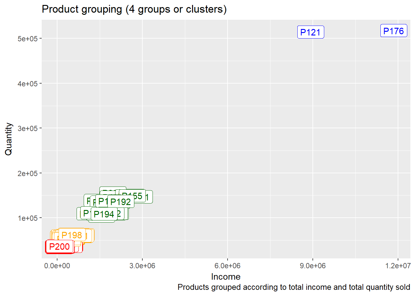
We can see that product P121 and product P176 are much more sold and brought much more income than the other products. The least sold and with the least income are products in the lower left corner (for example product P200).
If we seek similarities between products in the sense of locations where they are mostly sold, we get the following:
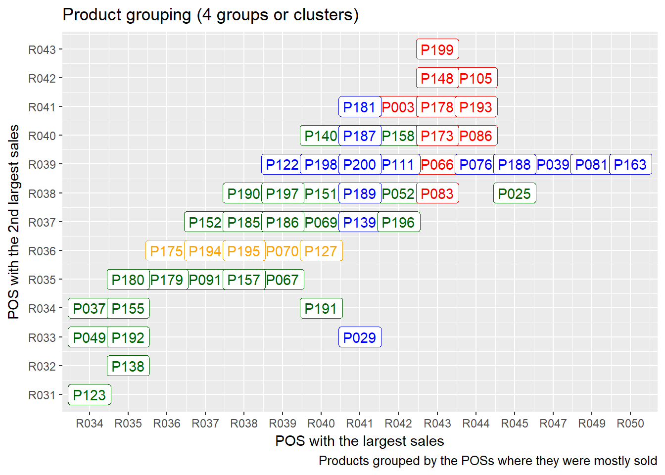
We see that there are products that are mostly sold at the very same point of sale (for example products P199, P148, P178, P173, P066, P083 are all mostly sold at R043).
Possible benefits from this information:
- increase marketing and offering of the most sought products at certain locations
- decrease marketing and offering of the least sought products at certain locations
- offer the most sought products at certain locations in a bundle or with a discount
Just as with the products, we can find similarities between POSs. First we investigate the similarities between POSs taking into account the total income and quantity sold.
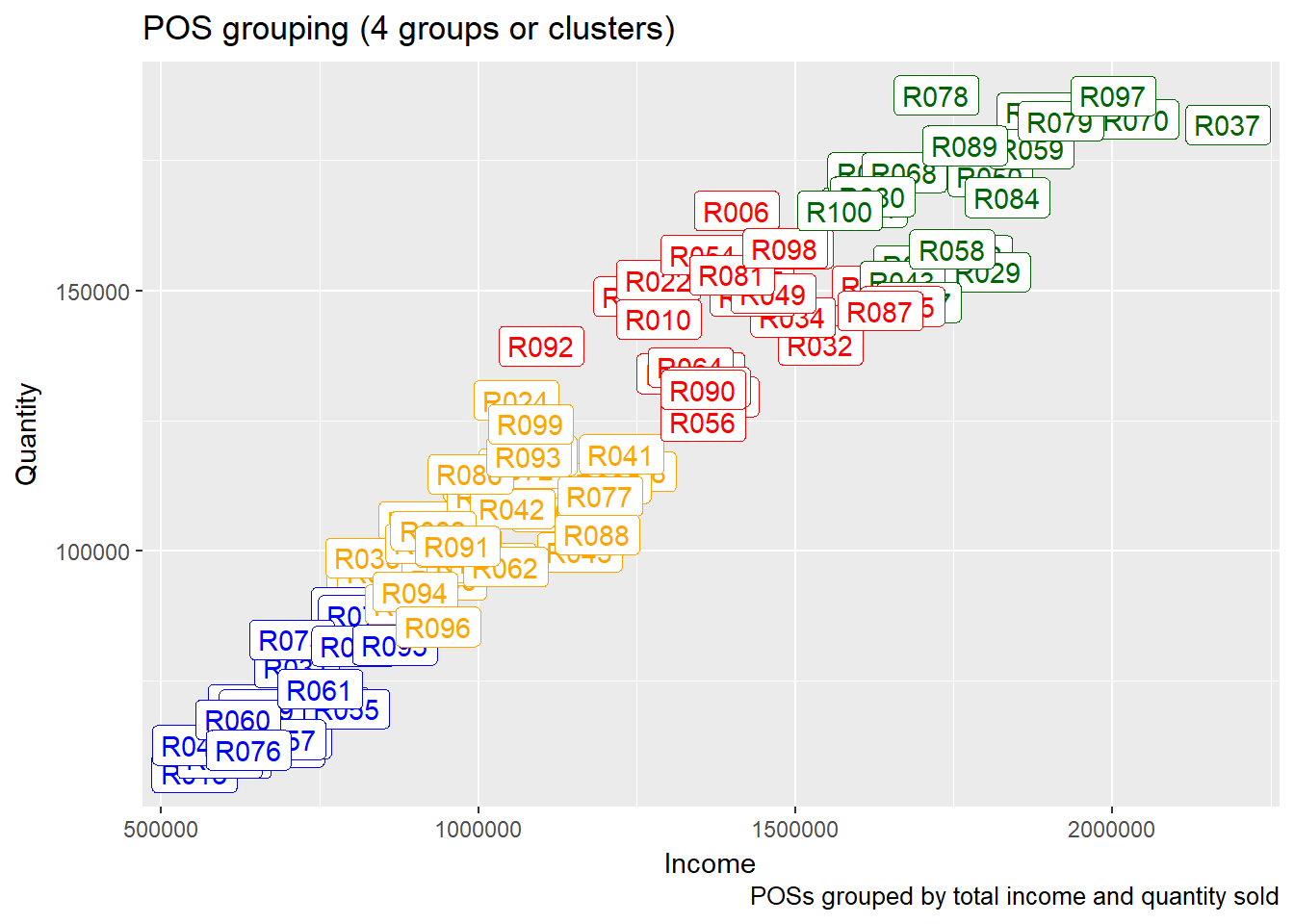
It is easily seen that there are groupings between points of sale: for example R078, R089 and R084 are very close (similar) with respect to income and quantities sold, while quite far (distant) from R076, R061, R060.
Possible benefits from this information:
- increase marketing and sales activities at the most profitable locations
- decrease marketing and sales activities at the least profitable locations
We can also find similarities between points of sale with respect to most sold product categories.
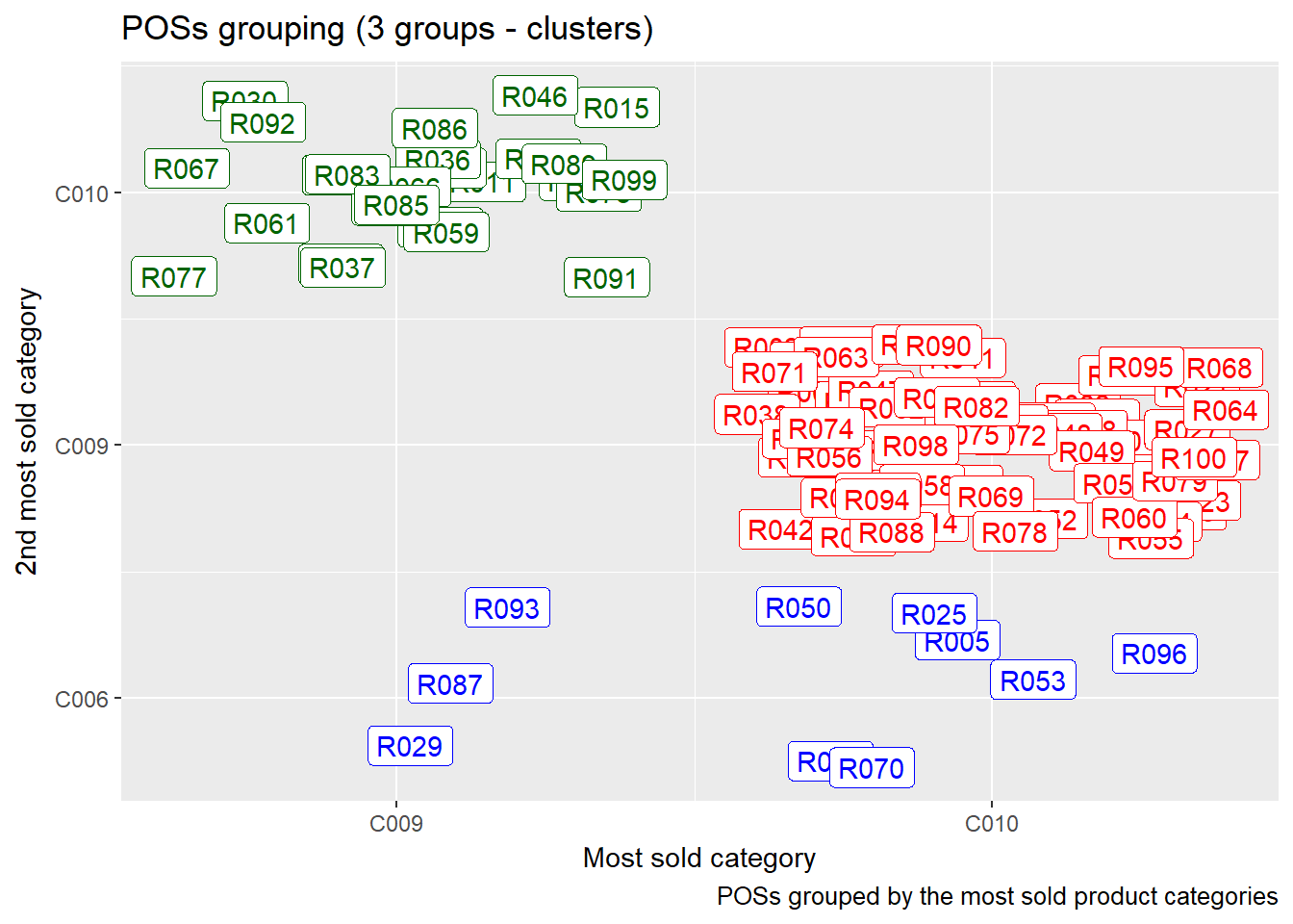
Possible benefits from this information:
- plan products distribution depending on the most and least sold product categories
- increase marketing and sales activities for the most sought product categories at certain points of sale
Just as we did with points of sale, we can investigate locations (cities, towns, provinces) to see if there are similarities with respect to average unit price and quantities sold.
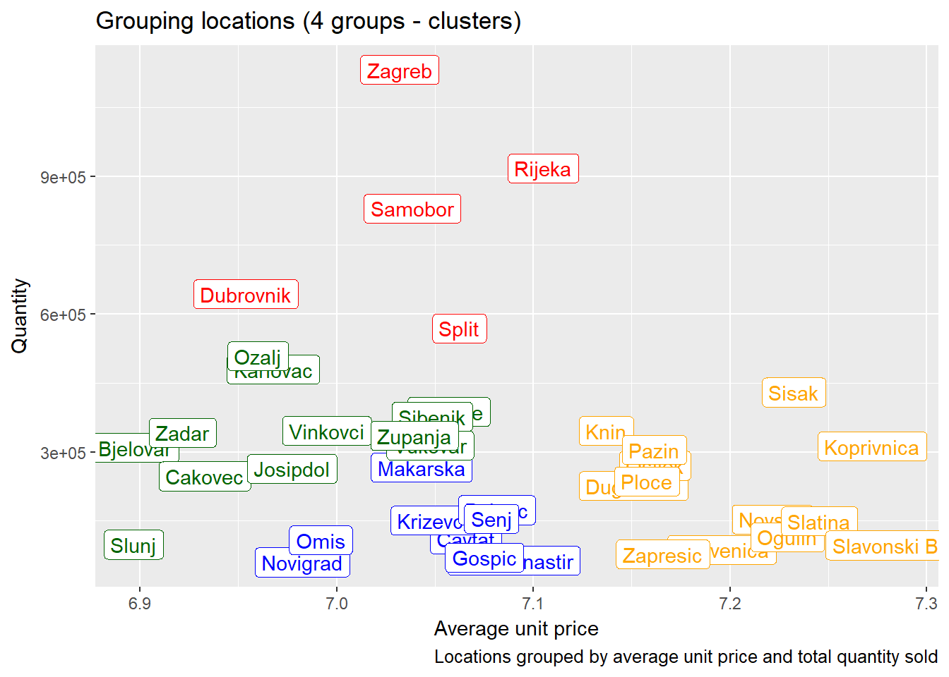
We see that for example Ogulin, Sisak and Koprivnica have lower total quantities sold and higher average product prices, while Dubrovnik, Samobor and Zagreb have higher quantities sold and and lower average product prices.
Possible benefits from this information:
- decrease prices in locations with higher average unit price to increase sales
- increase prices in locations with lower average unit price to increase profit
- increase marketing activities for high-end (more expensive) products in locations with high sales and lower average unit price
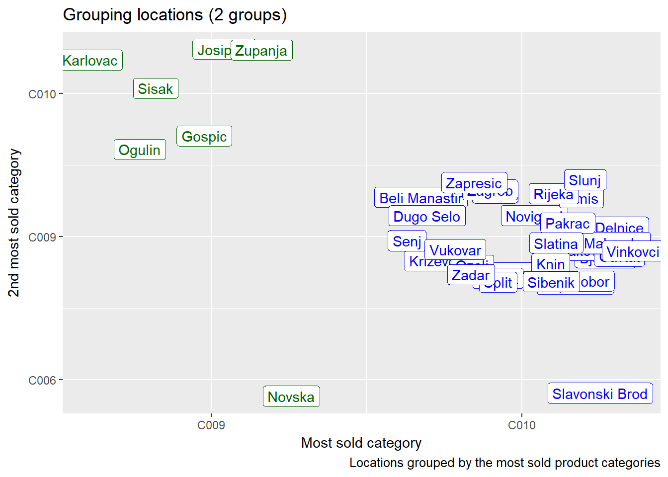
In the graph above we see that for example Zapresic, Vukovar and Slunj share the most sold product category and even the second most sold product category.
Possible benefits from this information:
- plan products distribution depending on the most and least sold product categories
- increase marketing and sales activities for the most sought product categories at certain locations
Classification
Existing data can also be classified to help making yes/no decisions. For example let’s classify the products with respect to their sales: are they sold above or below average (in terms of quantity), compared to all other products?
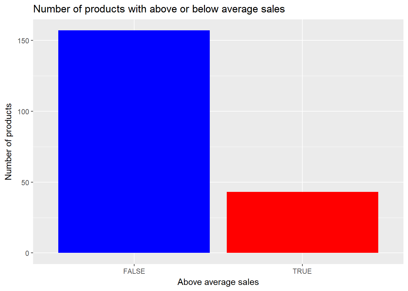
So most products are sold below average (in terms of quantity). What factors could influence this? From the data available, we pick the all the product related information: category, manufacturer and (average) unit price. These parameters will be used to build a classifier model and as future input for the model. The classifier model will output the product class – is it below or above the average sales quantity.
## Confusion Matrix and Statistics
##
##           Reference
## Prediction FALSE TRUE
##      FALSE    23    2
##      TRUE      3   10
##
##                Accuracy : 0.8684
##                  95% CI : (0.7191, 0.9559)
##     No Information Rate : 0.6842
##     P-Value [Acc > NIR] : 0.008114
##
##                   Kappa : 0.7022
##  Mcnemar's Test P-Value : 1.000000
##
##             Sensitivity : 0.8846
##             Specificity : 0.8333
##          Pos Pred Value : 0.9200
##          Neg Pred Value : 0.7692
##              Prevalence : 0.6842
##          Detection Rate : 0.6053
##    Detection Prevalence : 0.6579
##       Balanced Accuracy : 0.8590
##
##        'Positive' Class : FALSE
##
## [1] "ACCURACY: 0.87"Our model has a very high accuracy rate (87%) and we decide to use it to predict whether a new product produced by some (fixed) manufacturer and from some (fixed) product category will be sold below or above the average, depending only on its unit price.
## [1] "Will the sales be above the average (if the price is 16.00)? NO"## [1] "Will the sales be above the average (if the price is 15.00)? YES"We can conclude that the price 15.00 is the highest average unit price for this product that we expect to generate above the average sales.
Possible benefits from this information:
- for new products, predict their market behaviour, sales and other parameters compared to some group and adjust pricing and other variables to optimize the income or profit
Predicting the sales
Even more powerful than just classifying the data in two or more classes, we can use the existing data to build a model that predicts the sales depending on the given parameters. So if we give it the input parameters (product category, manufacturer, unit price), it will output the exact predicted sales quantity.
First we build the model and see how it behaves on the existing data (we use part of the existing data for building the model and part for testing the model):
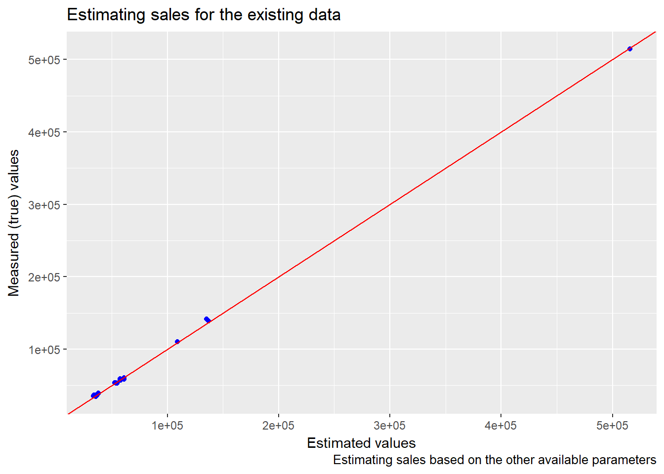
We see that the estimated values for the sales and the true/measured values for the sales lie very close to the red line which represents the perfect fit. Thus our model seems to be good (actually it’s almost perfect, but we’re working with simulated data and this kind of super fitting is very unlikely to happen on real data).
Let’s see how the model predicts the sales for a new product from a (fixed) product category made by a (fixed) manufacturer and different values of the unit price.
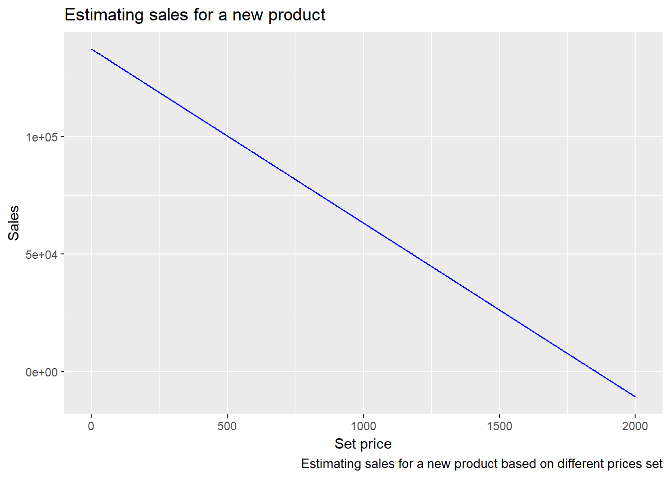
As expected, the estimated sales drops down as the price increases and is maximal close to 0. We can also see that the predicted sales drops to 0 at the price around 1.800.
An interested sales manager could then use another graph with calculated (or predicted) maximal profitability, see where these two graphs intersect and find the optimal price for a new (or even existing) product.
Possible benefits from this information:
- find the optimal pricing for a new product
Calculating the marketing effect
There is a saying that 50% of every marketing budget is wasted but one never knows which 50%. With data science the “wasted 50%” can be easily spotted.
As an example, we will use sample data consisting of 200 observations of sales as the target variable and TV, radio and newspaper promotion investing as the predictor variables, influencing the sales.
We will use the data, build a predicting model and test it on part of the existing data.
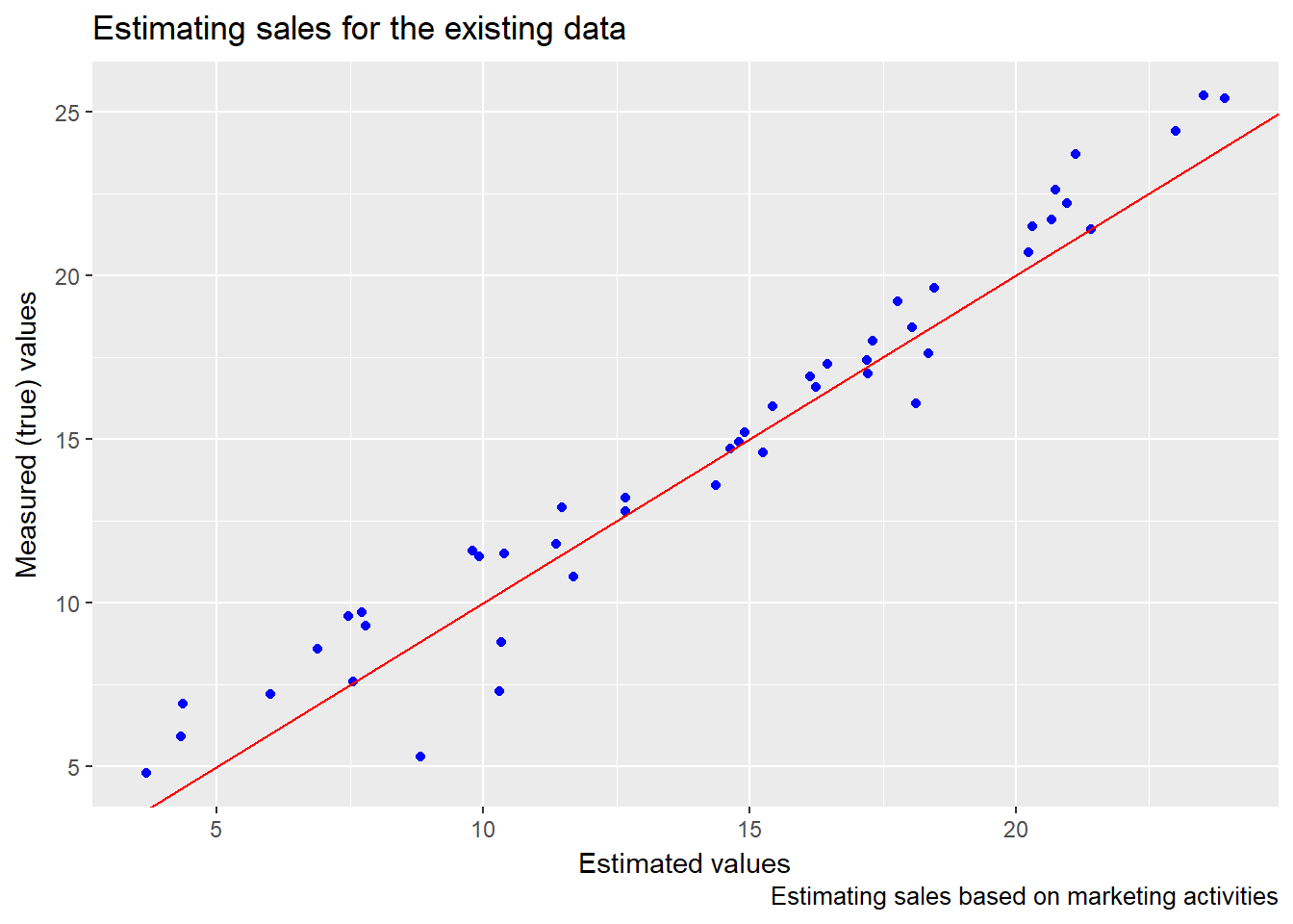
The red line, as before, represents the perfect fit in which all the predicted values are equal to all the measured values.
## [1] "Rounded mean square error: 0.269416957822519"## [1] "Coefficients for the predictor variables (TV, radio, newspaper):"## TV radio newspaper
## 0.74629300 0.54447603 -0.01637566The difference between our predicted values and the measured values is relatively small (rounded mean square error) which means that our model is pretty good in predicting the sales.
The coefficient by the newspaper variable is very small (around 0.01). This (together with some other arguments) means that newspaper promotions are very slightly, almost not at all, influencing the sales. This is an important discovery because it basically means that we can decrease or even completely remove newpaper investing from our marketing activities. Let’s see what happens if we completely remove the newspaper from investment.
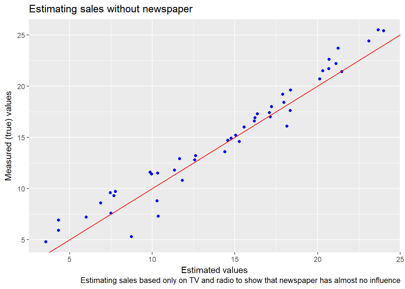
## [1] "Rounded mean square error: 0.267409702787592"The difference between the predicted values and the measured values is practically the same as when we used the newspaper parameter.
Thus we can conclude that stopping investing in newspaper promotions and redirecting the budget to TV and radio will reduce costs and increase the marketing effect. We’ve found the “50% wasted” marketing budget. 🙂
Possible benefits from this information:
- find the optimal marketing mix and optimize the promotion effect
Conclusion
Data science provides many different tools and approaches to analyze data and make educated business decisions.
Are you analyzing your data? 😉
Wow Good Article, can i share it?
Of course! Thanks for the comment!
I am glad to found your blog and read your article, very informative. Keep writing, Regards
Thanks! I’m not very active in writing, but I’ll try to do it more… 🙂
your post so informative, love your writting style, thank for sharing this